Diffusion Without Bulk Flow
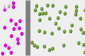
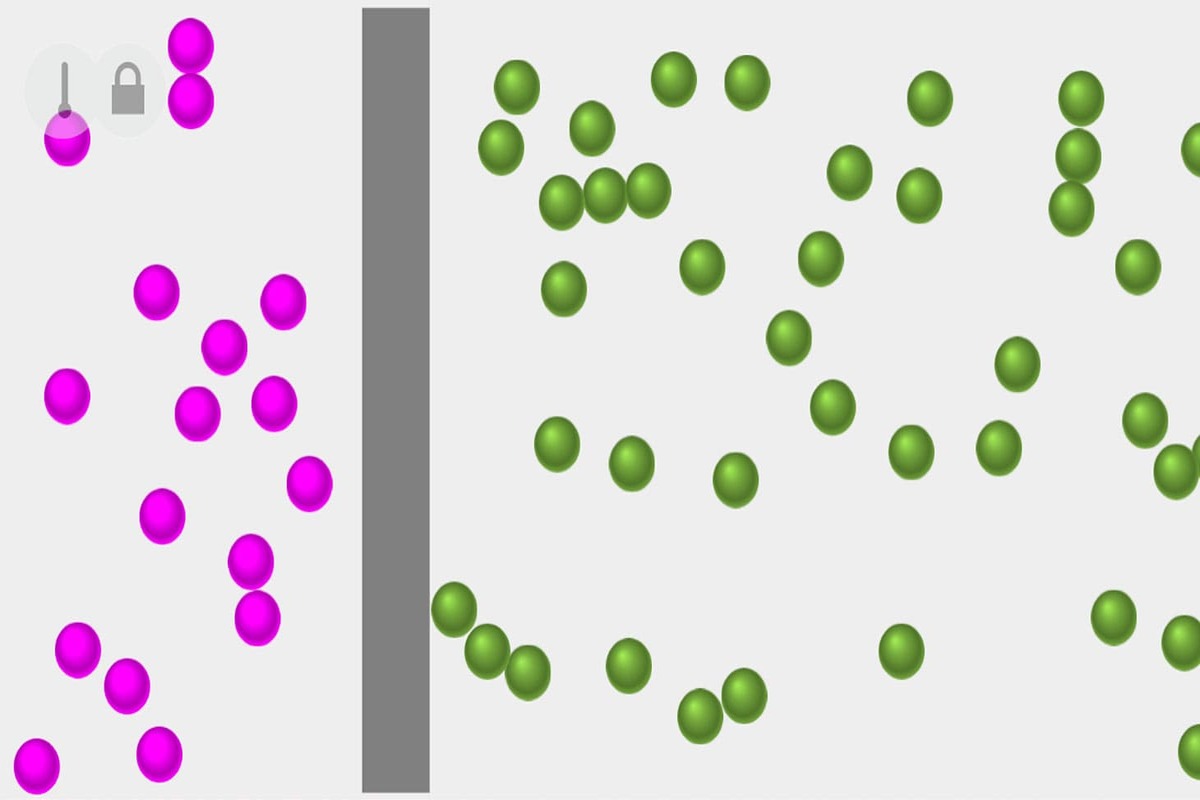
Diffusion moves molecules because random thermal motion causes a net spread from regions of higher concentration to regions of lower concentration. No bulk flow is required: the fluid can remain still while molecules keep jostling each other. A useful mental model is a crowd of walkers who constantly change direction; if one side has more people, more walkers cross the middle from that side than from the other side, even though nobody is “pushing” them in one direction.
In physics terms, diffusion is driven by concentration gradients, not by pressure gradients alone. In chemistry and biology, the same idea shows up as mass transport through membranes, across cell layers, and within porous tissues. The rate depends on how fast molecules move (linked to temperature and molecular size) and how far they must travel (linked to geometry and thickness). When diffusion is the main transport mechanism, the time scale grows quickly with distance, which is why thin barriers matter so much.
Diffusion also interacts with other processes that can mimic or mask it. Binding to surfaces, chemical reactions, and active transport can change the local concentration profile, which then changes the diffusion flux. That coupling is why two systems with the same membrane thickness can show different “diffusion-like” behavior.
Common Misunderstandings
People often treat diffusion as if it were a slow “leak” that only happens when fluid is moving. In reality, diffusion can dominate even when the bulk fluid velocity is zero, because molecular motion continues. Another frequent mistake is assuming that diffusion always moves in the direction of decreasing concentration everywhere at once; instead, the local flux depends on the local gradient, which can vary across space and time.
Readers also confuse diffusion with convection. Convection transports material because the fluid itself moves; diffusion transports material because molecules move relative to the fluid. In many real systems, both occur together, and the balance depends on length scale, viscosity, and typical velocities. A small channel with slow flow can look diffusion-dominated, while a larger vessel with faster flow can look convection-dominated.
Supporting technologies and dependencies shape what you observe. In lab measurements, diffusion coefficients are often inferred from concentration-time curves using methods like diffusion cells or fluorescence recovery after photobleaching (FRAP). In tissue or membrane contexts, the “effective” diffusion coefficient can differ from the free-solution value due to tortuosity, binding, and obstacles. When a model uses an effective diffusion coefficient, it usually hides multiple microscopic effects inside one parameter.
Temperature and molecular size matter because they change molecular mobility. For many small molecules in water, diffusion coefficients are on the order of 10-9 to 10-10 m2/s, while larger macromolecules diffuse more slowly. Those ranges are broad enough that you should check the specific molecule and medium rather than copying a generic number from a blog post.
How To Predict Diffusion Dominance
Use a transport timescale
A practical way to decide whether diffusion can act on a given timescale is to compare the characteristic diffusion time to the process time. Diffusion time grows with the square of distance, so doubling the thickness makes diffusion about four times slower. For order-of-magnitude thinking, you can use the idea that the distance scale relates to time through diffusion coefficient and geometry; the exact prefactor depends on boundary conditions.
As a concrete aside, if a small molecule has a diffusion coefficient near 2×10⁻⁹ m2/s in water, then crossing 100 micrometers (1×10⁻⁴ m) takes on the order of seconds, while crossing 1 millimeter (1×10⁻³ m) takes on the order of hundreds of seconds. Those are rough estimates, but they match the intuition that diffusion struggles across thick barriers. In tissues, the effective diffusion coefficient can be lower, which pushes those times upward.
Check the concentration gradient
Diffusion flux depends on how steep the concentration gradient is, not on the absolute concentration alone. If a system maintains a steep gradient—such as a fresh supply on one side of a membrane and a sink on the other—diffusion can keep moving material at a near-steady rate. If the gradient relaxes quickly, the flux drops even if the medium remains unchanged.
In practice, you can look for evidence of gradient maintenance. For example, a well-stirred reservoir on one side of a membrane acts like a boundary condition that holds concentration nearly constant. A sink that removes molecules (through metabolism, binding, or sampling) can keep the downstream concentration low. When neither side is a sink, the gradient shrinks, and diffusion slows.
Account for obstacles and binding
In porous media and biological tissues, molecules encounter obstacles that slow transport. Tortuosity describes how convoluted the pathways are compared with straight-line distance. Binding to extracellular matrix components or cell surfaces can also reduce the fraction of molecules that remain free to diffuse, which lowers the effective diffusion coefficient.
When you see a model using an “effective diffusion coefficient,” treat it as system-specific. A value measured in one tissue region or at one hydration level may not transfer to another. If a study reports an effective coefficient, check the measurement method and the conditions; FRAP, diffusion chamber experiments, and tracer studies can yield different values because they probe different length scales.
Separate diffusion from flow with dimensionless checks
When bulk flow exists, diffusion competes with convection. A common decision tool is to compare characteristic diffusion and convection effects using a dimensionless ratio that scales with velocity, length, and diffusion coefficient. If the ratio indicates convection dominates, diffusion alone cannot explain transport; if diffusion dominates, concentration gradients drive the motion even when flow is small.
One mild frustration: many simplified explanations skip the length scale. The same flow speed can be diffusion-dominated in a thin layer and convection-dominated in a thick region. If you are reading a paper, track the length scale used to define the ratio, not just the reported velocity.
Case Examples From Real Systems
Example 1: Gas exchange across a thin barrier. Consider oxygen moving from an alveolar air space into blood across a thin membrane. The bulk air and blood motions exist, but the key step is that oxygen concentration is higher on the air side and lower on the blood side. Diffusion carries oxygen across the barrier while the gradient is maintained by ventilation and blood perfusion. If the barrier thickens or the effective diffusion coefficient drops due to tissue changes, the diffusion time increases sharply because distance enters strongly.
Example 2: Drug penetration through a gel layer. Imagine a topical formulation spreading into a hydrogel that contains a drug. If the gel is initially drug-free and the formulation maintains a higher drug concentration at the surface, diffusion drives drug into the gel. As the drug front advances, the gradient at the front decreases, slowing further penetration. If the drug binds to gel components, the effective diffusion coefficient decreases, and the concentration profile becomes more front-like rather than uniform.
Diffusion vs Convection Checklist
| Question | If Yes, Expect | If No, Expect | What To Check |
|---|---|---|---|
| Is bulk fluid velocity near zero? | Diffusion can dominate | Convection may contribute | Velocity measurements or assumptions about “still” fluid |
| Is the barrier thin? | Diffusion acts on relevant timescales | Diffusion slows dramatically | Distance scale used in the model |
| Does a sink maintain a gradient? | Sustained diffusion flux | Flux drops as gradients relax | Boundary conditions: reservoirs, mixing, removal |
| Are obstacles or binding present? | Effective diffusion coefficient decreases | Transport closer to free diffusion | Tortuosity, binding kinetics, reported measurement method |
If you want a step-by-step decision path, start by identifying the length scale and the timescale of the process, then estimate whether diffusion can traverse that distance before the process ends. Next, confirm whether concentration gradients are maintained by boundary conditions. Finally, check whether the medium requires an effective diffusion coefficient rather than a free-solution value.
Practical Common Mistakes
One mistake is using a diffusion coefficient from water for a complex medium without adjustment. Even small changes in temperature or viscosity can shift diffusion rates, and tissues add tortuosity and binding. Another mistake is treating diffusion as purely one-dimensional when the geometry forces lateral spreading. In a real membrane or tissue slab, edge effects can dominate when the lateral dimensions are comparable to the thickness.
People also misread experimental outputs. FRAP, for example, reports recovery dynamics that depend on both diffusion and binding/unbinding, and the inferred diffusion coefficient depends on the analysis model. A paper might report “diffusion coefficient” while the underlying fit includes reaction terms, which changes interpretation. I once saw a lab notebook entry dated 2024-11-03 where the same sample produced two different diffusion estimates because the fitting window was changed; that kind of sensitivity is common.
Another error is ignoring units and scaling. Diffusion coefficients use m2/s, while distance might be reported in micrometers or millimeters. Mixing units can shift timescales by orders of magnitude. If you are using a spreadsheet, double-check conversions; Excel formulas can silently propagate wrong units, and the graph still looks “reasonable,” which is maddening.
FAQ
Does diffusion stop when fluid is still?
No. Diffusion continues because molecules undergo random thermal motion even when the bulk fluid velocity is zero. What changes is the net flux direction and magnitude as the concentration gradient evolves.
How is diffusion different from osmosis?
Diffusion describes net movement of particles down a concentration gradient. Osmosis is diffusion of water driven by differences in solute concentration across a semipermeable barrier, so it depends on membrane selectivity and water transport.
Why does diffusion slow over longer distances?
Diffusion time scales strongly with distance, so thicker barriers require more time for the same fraction of molecules to traverse. Obstacles and binding in real media can further reduce the effective diffusion coefficient.
Can diffusion create a steady concentration profile?
Yes when boundary conditions maintain gradients, such as a constant source on one side and a sink on the other. Without gradient maintenance, diffusion tends to reduce the gradient and the net flux declines.
What measurements estimate diffusion without bulk flow?
Diffusion chamber experiments, tracer studies in quiescent media, and imaging methods like FRAP can estimate diffusion under controlled conditions. Interpretation depends on whether binding or reactions are included in the analysis model.
Author's Insight
Diffusion without bulk flow is best understood as a consequence of random molecular motion plus a concentration gradient. The same physical idea shows up across scales: molecules crossing membranes, solutes spreading through gels, and gases moving across thin exchange layers. Real systems often require an effective diffusion coefficient because tortuosity and binding alter transport compared with free solution. When you read diffusion results, track the length scale, the boundary conditions, and the analysis model used to infer the coefficient; those details determine whether the number describes free diffusion or a coupled transport process.
Key Takeaways
- Diffusion moves molecules down concentration gradients without requiring bulk fluid motion.
- Diffusion rate depends on molecular mobility, distance, and whether gradients are maintained by sources and sinks.
- Biological and porous media often need an effective diffusion coefficient due to tortuosity and binding.
- When flow exists, diffusion and convection compete; use length scale and timescale to judge which mechanism dominates.
- Interpret diffusion measurements by checking the method and the model assumptions, since binding and geometry can change the inferred “diffusion coefficient.”